

Can you really trust a query you run once a day?
Insights on how to set the number of prompts and queries when measuring GEO data.
Chris
A heated debate has emerged in the AI search visibility industry: "Measurement that runs a prompt only once a day cannot be trusted." Chainshift answered this question with measured data from the Korean market, not simulations or estimates. We ran a campaign that actually executed the same prompt set 10 times a day alongside a campaign that executed it once a day over the same period and compared the measured values directly. On top of that, we added a resampling experiment that keeps only one random run out of the 10 runs on the same day as a cross-check.
One thing should be clear up front. This analysis does not show that responses to individual prompts are stable. When the same prompt was run repeatedly, the responses and cited sources did change. However, when about 635 prompts and 5 models were aggregated at the portfolio level, we observed no practically meaningful difference in visibility or citation source mix between measuring once a day and 10 times a day.
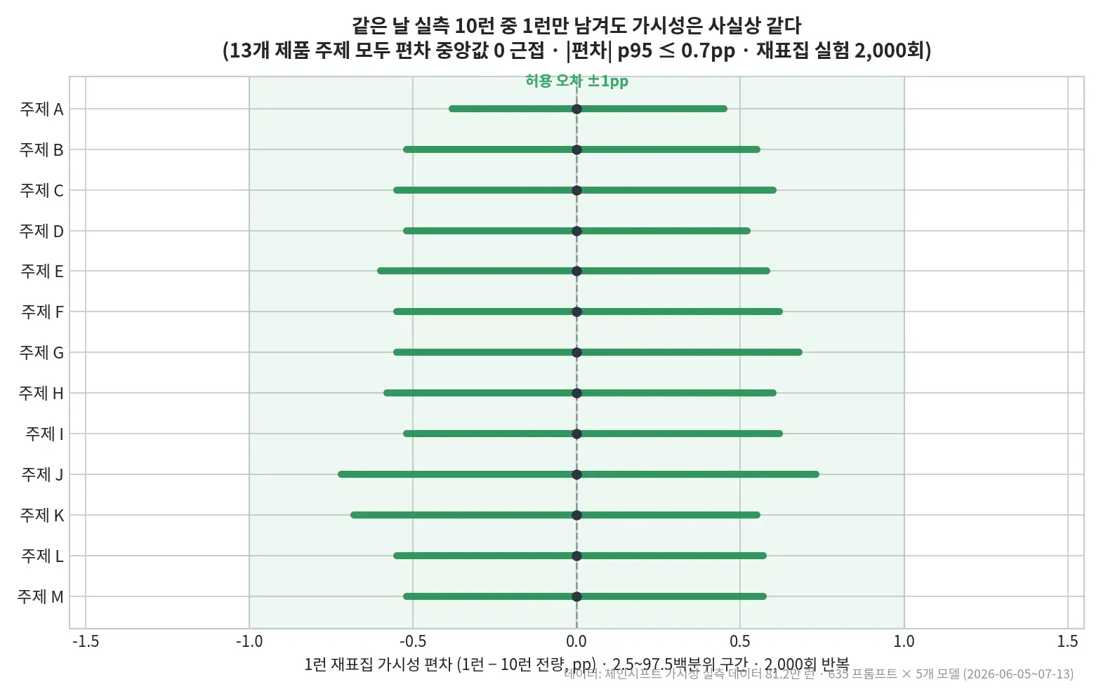
For ratio KPIs aggregated at the portfolio level, measuring once a day and 10 times a day produced practically similar results. The total variation distance of the citation source mix was only 2.3pp, with an effect size (Cramér's V) of 0.025. Visibility differed by 1.1pp in the measured side-by-side comparison (topic rank correlation ρ=0.91). In the resampling experiment that keeps only 1 of the 10 runs on the same day, the median deviation was close to 0 for all 13 topics, and the 95th percentile of absolute deviation was at most 0.7pp.
That said, not every metric behaves this way. Discovery metrics, which ask "how many sources do we find?", are strongly affected by the number of runs. Running 10 times a day captured 2.1x more unique URLs and 1.7x more unique hosts than running once. So this result should not be read as "once a day is enough for every measurement." It should be read as evidence that portfolio-level ratio KPIs and individual-prompt or discovery metrics need different collection designs.
1. The trigger: the industry's long-standing worry, "Is once a day enough?"
Ask ChatGPT the same question twice and you get two different answers. LLMs are non-deterministic systems that sample tokens probabilistically. This property raises a fundamental question for every tool that measures AI search visibility: "Can we trust a number obtained by running a prompt only once a day?"
This question has recently split the global AEO/GEO industry into two opposing camps. One side criticizes that "many GEO platforms do not sample enough and leave data with unacceptable margins of error." According to Evertune's analysis, repeating a single prompt only 5 times leaves a margin of error of ±27pp in the brand visibility score, and it takes 100 repetitions to narrow it to around ±6pp. At the level of individual prompts, this point is statistically valid.
On the other side is Profound, the best-known proponent of running prompts once a day. Profound's Josh Blyskal pushed back by analyzing about 1 million AI responses and 6.6 million citations. Running a 753-prompt portfolio across 7 models once a day and 10 times a day in parallel for 14 days, citation share came out at 10.24% and 9.99% respectively, a difference of only 0.25pp. To be fair, Profound did not say repetition has no effect at all. In the same analysis, 10 repetitions reduced the range of daily citation share fluctuation from about 0.36pp to 0.21pp, roughly 40%. The key point is that because the fluctuation was small to begin with, the absolute difference at the portfolio level was only 0.25pp. His argument is simple: individual prompts may look unstable, but the prompt portfolio itself is already a powerful averaging device.
As Josh Blyskal of Profound puts it, refreshing the wrong keyword set more often does not make an SEO rank tracker more representative of the market, and the same holds for prompt tracking.
So who is right? And does this debate hold the same way in the Korean market, with Korean-language prompts and Korean brands? Instead of guesses or simulations, Chainshift decided to find out with measured data from actually running both approaches.
2. Experiment design: measured side-by-side operation, plus a cross-check that leaves no room for chance
This analysis does not start from a simulation. Chainshift ran a campaign that actually executed the same prompt set 10 times a day and a campaign that executed it once a day over the same period. We did not mathematically estimate "what if we had run it 10 times"; we ran both and compared the measured values.
Even this kind of measured comparison has pitfalls. If the measurement periods do not line up, changes in the market itself (period effects) can look like frequency effects, and if the prompt sets differ, the comparison does not hold in the first place. So we kept the measured side-by-side comparison at the center and designed a two-layer system with a cross-check to reinforce it.
| Axis | Question | Design |
|---|---|---|
| A. Measured side-by-side comparison (main analysis) | Does data from actually running 10 times a day differ from data from running once a day? | A 10-runs/day campaign and a 1-run/day campaign with the same prompts, run in parallel — controlled to 19 overlapping days · 635 common prompts · 5 models (ChatGPT · Gemini · Google AI · AI Overviews · Perplexity) |
| B. Resampling experiment (cross-check) | Is visibility the same if we keep only 1 of the 10 runs on the same day? | From the measured 10-runs/day data, randomly draw 1 run per cell (day × prompt × model), repeated 2,000 times — same dates, so period confounding is blocked |
We are also transparent about sample size. After applying the control conditions (common period · 635 common prompts · the same 5 models), the citation data collected by the two campaigns came to 2.535 million and 549,000 rows respectively, about 3.08 million rows in total. After also applying the valid-label condition, the final analysis sample was 2.81 million rows. For the visibility analysis, we used a separate measurement set of 812,000 runs.
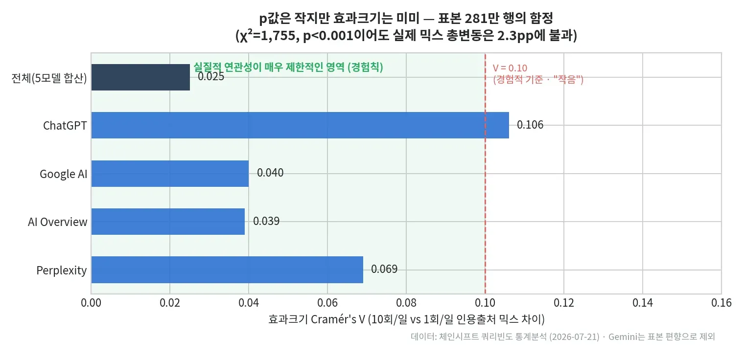
One point about statistical treatment is worth noting here. When the sample grows to millions of rows, even tiny differences with almost no practical meaning can produce very small p-values. With large data, you need to check not just "is there a difference?" but "how big is that difference, really?" In this analysis, we did not draw conclusions from p-values alone and interpreted the results centered on effect sizes (Cramér's V, Cliff's δ) and confidence intervals. Citation rows from the same prompt also resemble each other (cluster correlation), so we calculated confidence intervals for the differences with 2,000 prompt-level cluster bootstrap iterations. For the p-values of multiple tests across 14 source types, we applied Benjamini-Hochberg FDR correction at 5% to control false discoveries from multiple comparisons. For equivalence, we set predefined practical tolerance margins (±1pp, secondary ±2pp) and used TOST logic to check whether the 95% interval of the deviation falls within the margin.
3. Result 1: Even with 10x the queries, the citation source mix was practically similar
We compared the composition of the source types AI answers cite (14 types including social media, blogs, portals, marketplaces, and official sites) using the measured data from the 10-runs/day campaign and the 1-run/day campaign that we actually ran in parallel. Strictly speaking, this comparison is of the source type composition aggregated over all collected citation rows.
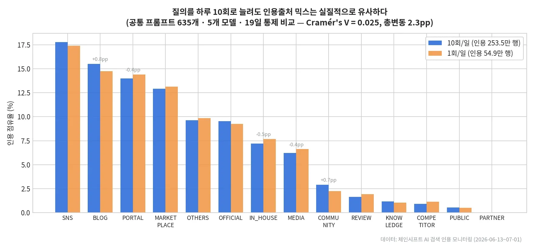
The chi-square test of homogeneity gives χ²=1,755, p<0.001, detecting a "statistically significant difference." But this is exactly the large-sample pitfall described above. In terms of effect size, Cramér's V = 0.025, which indicates very limited practical association even against the commonly used rule of thumb (treating values below 0.10 as negligible). The total share that would need to move to make the two distributions match (total variation distance, TVD) is 2.3pp, within the predefined tolerance margin, and the Jensen-Shannon distance is only 0.028.
Breaking it down by type gives the same picture. Based on bootstrap confidence intervals, some types show significant differences, such as BLOG (+0.75pp), PORTAL (−0.42pp), IN_HOUSE (−0.48pp), and COMMUNITY (+0.67pp), but their absolute size is around 1pp in every case. Even after running 635 prompts on 5 models 10 times a day for 19 days and collecting millions of citation rows, the result is practically similar to the mix structure drawn by the once-a-day campaign.
| Metric | Value | Interpretation |
|---|---|---|
| χ² (test of homogeneity) | 1,755 (p<0.001) | Sample of 2.81M rows → p-value alone is not enough to decide |
| Cramér's V | 0.025 | Very limited practical association against the rule of thumb |
| Total variation distance (TVD) | 2.3pp | Total share that would need to move across all 14 types |
| Jensen-Shannon distance | 0.028 | Information-theoretic distance between distributions, close to 0 |
| Largest difference by type | ~around 1pp | Significant, but of limited practical meaning |
To be honest about one thing: this comparison (A) is an observational comparison in which the two campaigns may also differ in collection settings other than query frequency. So we do not interpret the observed 2.3pp causally as a pure frequency effect. Isolating the effect of frequency alone is the job of the resampling experiment in the next section.
4. Result 2: Portfolio-level visibility did not depend much on run frequency
The metric more teams check every day than the citation source mix is visibility: the share of AI answers that mention our brand. In this analysis, we ran an even stricter check to reduce the limits of comparing across campaigns.
First, to be clear: this experiment is also based entirely on real operating data. Chainshift actually ran a campaign executing the same prompt set 10 times a day and a campaign executing it once a day. In addition, from the measured 10-runs/day data, we ran a resampling experiment 2,000 times that virtually reproduces once-a-day measurement by randomly selecting only 1 of the 10 runs for each day, prompt, and model.
We cross-checked the results from three perspectives: the real 10-run campaign, the real 1-run campaign, and 2,000 resampling experiments using the real 10-run data. In particular, the resampling experiment uses only measured values from the same dates, so period effects such as market changes or the passage of time are removed. This design lets us isolate the measurement error that arises from sampling 1 run instead of averaging 10.
The results were highly consistent. Across 2,000 resamples, the median deviation was close to 0 for all 13 product topics, and the 95th percentile of absolute deviation was at most 0.7pp, below 1pp for every topic. In other words, visibility from running 10 times a day and visibility from running once a day were effectively the same within the range of statistical noise.
In actual operation, a simple before-and-after comparison around the point when collection frequency changed from 10 times a day to once a day showed a +1.0pp difference in visibility. At first glance, it is easy to read this as "reducing collection frequency changed visibility." But when we widened the comparison period a little, the difference grew to +2.2pp. If collection frequency were the cause, the difference should stay at a similar level when the comparison period changes. This shows that the passage of time itself, not collection frequency, had the effect. Indeed, over the full period, visibility trended gradually downward from 82.5% in early June to 79% in July.
In contrast, the resampling experiment, which used only measured data from the same dates, showed almost zero visibility deviation. Matching the dates exactly removes external factors such as market changes and seasonality, so the stability of aggregation by number of samples can be checked in isolation. This result supports that the +1.0pp difference shown earlier came from a period effect, not collection frequency.
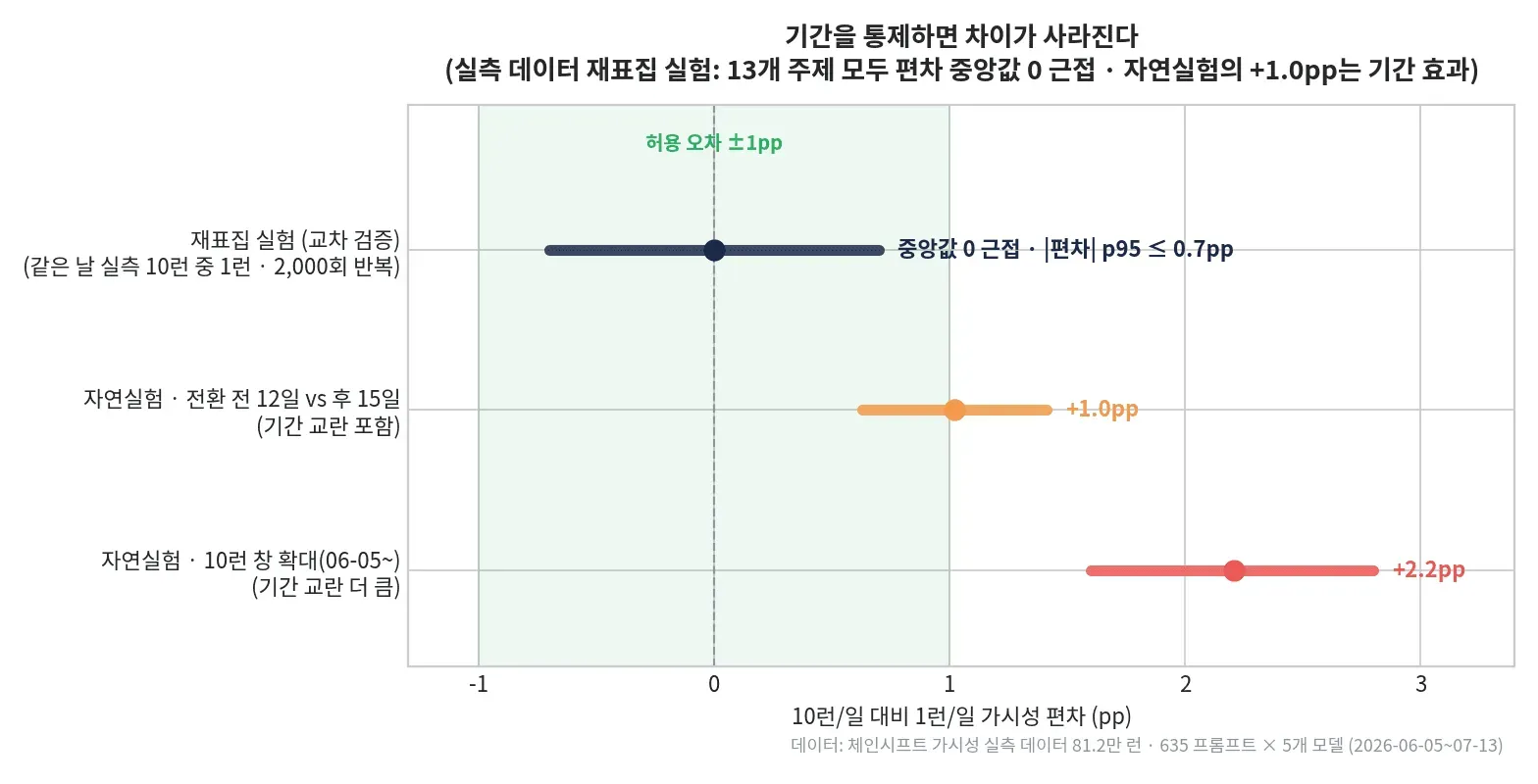
Why this matters in practice: concluding that a KPI movement is a policy effect just because it moved when the collection policy changed can lead to wrong decisions. When interpreting time series data, you must always control for trends and period effects together.
Finally, the two campaigns actually run in parallel showed the same conclusion. Compared on the same labeling criteria and 635 common prompts, visibility was 80.4% for the 10-runs/day campaign and 81.5% for the 1-run/day campaign, a difference of 1.1pp, with a visibility rank correlation of ρ=0.91 across the 13 topics. In other words, in real operation too, the 10-times-a-day and once-a-day campaigns were measuring effectively the same visibility.
5. But not all metrics are the same: "discovery" is a function of query volume
If you stop reading here, it is easy to jump to the conclusion "so we should just cut it down." But the data also shows a warning in the opposite direction.
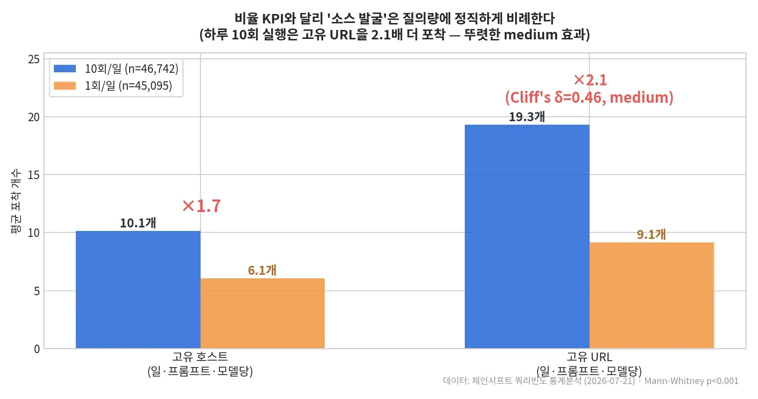
Diversity and discovery metrics are strongly affected by the number of runs. Per (day · prompt · model), the 10-runs/day campaign captured 1.7x more unique hosts (10.1 vs. 6.1) and 2.1x more unique URLs (19.3 vs. 9.1) than the 1-run campaign. The effect size from the Mann-Whitney test, Cliff's δ, was 0.43–0.46, a clear medium effect, unlike in the mix comparison.
The reason for this difference is intuitive. LLMs cite a slightly different combination of sources on every run, so the more runs there are, the longer the list of "sources that have been cited at least once" grows. Ratios (composition) converge quickly with repeated runs, but unique counts keep growing as a function of collection volume. In fact, 65% of the citation hosts observed during the analysis period first appeared after the first day of collection. The pool of citation sources in the AI answer ecosystem is not static; it is a dynamic system with new faces flowing in every day.
The implication is clear. If you want to capture without gaps "which new community posts and which influencer content AI has started citing about our brand," and if you want to detect spikes such as a sharp drop in visibility on a particular day (during the analysis period there was a single-day event where visibility on Perplexity fell to 57%), you should not cut collection volume.
Another practical implication concerns benchmarking. Diversity metrics such as "number of cited sources per answer" can differ by a factor of 2 depending on query design, so comparing absolute values across tools or periods with different query volumes is a mistake. If different tools show different "numbers of discovered sources," it is more likely simply because one sent more queries, not because the market differs.
6. Conclusion: the question is not "how many times you run it" but "what you are measuring"
The conclusion of this analysis in one sentence: the right answer to the query frequency debate depends on the type of metric.
| Measurement purpose | Metric type | Recommended collection design | Evidence |
|---|---|---|---|
| Regular KPI reports (visibility · mix · share · mention rate) — aggregated over a portfolio of hundreds of prompts × multiple models | Ratio | Once-a-day measurement is similar to 10 times a day (1/10 the cost) | Resampling median deviation near 0 · absolute deviation p95 at most 0.7pp, 1.1pp difference between measured campaigns |
| Discovering new sources and influencers | Discovery | Maintain or expand collection volume | 65% of sources newly appeared during the period, 10/day captured 2.1x unique URLs |
| Detecting spikes and issues | Event | Collect every day without gaps | A single-day event (Perplexity's sharp drop to 57%) cannot be observed if collection has gaps |
| Managing targets for low-visibility topics | Ratio (high variance) | Once a day is possible, but apply a ±2pp margin | Topics in the 60–75% visibility range have wide deviation intervals |
| Comparing diversity metrics across tools or periods | Discovery | Compare only after standardizing query volume | Absolute values differ 2x depending on query design |
However, the conclusion that "once a day is similar" has a clear scope. What this result supports is the condition of regular KPIs aggregated over a portfolio of about 635 prompts across 5 models. It cannot be generalized as-is to campaigns with only a few dozen prompts, single-model measurement, diagnosis at the individual prompt level, same-day sudden-change detection, or environments with different industries and languages. Instability at the individual prompt level is real; it is the portfolio, as an averaging device, that absorbs it.
[Chainshift offers an API on Chainshift Platform that lets marketers collect AI answers and measure visibility even without the Chainshift dashboard, and an MCP is on the way. If you want to measure GEO for a variety of purposes like those above, contact us and we will get back to you quickly. :)]
This result also points in the same direction as Profound's analysis that "the difference between once and 10 times a day is only 0.25pp." Results obtained from a different market (Korea), a different prompt set, and an independent dataset converged on the same conclusion. Of course, the instability at the individual prompt level that Evertune pointed out also exists. For low-visibility topics (the 60–75% visibility range), the deviation was relatively large. But the solution is not necessarily to run the same prompt dozens or hundreds of times. Designing portfolio-level aggregation, a sufficient observation period, and a tolerance suited to the purpose together solves most of the problem. The two camps' claims do not actually conflict: Evertune is talking about ratio estimation error for individual prompts, and this analysis is talking about the stability of large-scale portfolio aggregation.
In the end, when evaluating a measurement tool, "how many times a day do you run it?" is an important question, but it is not the most important one. The more important questions are these two:
-
Is this metric a ratio metric or a discovery metric? And does the collection design fit that purpose?
-
How well does this prompt set represent the questions real customers ask AI?
The second question matters most. No matter how much data you collect or how sophisticated the statistics, if you measure prompts that do not represent reality, the results cannot represent reality either. Precise analysis only shows good data more accurately; it cannot turn the wrong question into the right one.
Chainshift will continue to verify and share AI search measurement methodology through real data from the Korean market, not mere claims or intuition.